
Definitions of Various Terms:
(1) Sample space:
The set of all possible outcomes of a trial (random experiment) is called its sample space. It is generally denoted by S and each outcome of the trial is said to be a sample point.
(2) Event:
An event is a subset of a sample space.
► Simple event: An event containing only a single sample point is called an elementary or simple event.
► Compound events: Events obtained by combining together two or more elementary events are known as the compound events or decomposable events.
► Equally likely events: Events are equally likely if there is no reason for an event to occur in preference to any other event.
► Mutually exclusive or disjoint events: Events are said to be mutually exclusive or disjoint or incompatible if the occurrence of any one of them prevents the occurrence of all the others.
► Mutually non-exclusive events: The events which are not mutually exclusive are known as compatible events or mutually non exclusive events.
► Independent events: Events are said to be independent if the happening (or non-happening) of one event is not affected by the happening (or non-happening) of others.
► Dependent events: Two or more events are said to be dependent if the happening of one event affects (partially or totally) other event.
(3) Exhaustive number of cases:
The total number of possible outcomes of a random experiment in a trial is known as the exhaustive number of cases.
(4) Favourable number of cases:
The number of cases favourable to an event in a trial is the total number of elementary events such that the occurrence of any one of them ensures the happening of the event.
(5) Mutually exclusive and exhaustive system of events:
Let S be the sample space associated with a random experiment. Let A1, A2, …..An be subsets of S such that
(i) Ai ∩ = φ for i ≠ j and (ii) A1 ∪ A2 ∪ ... ∪ An = S
Then the collection of events A1, A2, ....., An is said to form a mutually exclusive and exhaustive system of events.
If E1, E2, ..., En are elementary events associated with a random experiment, then
(i) Ei ∩ Ej = φ for i ≠ j and (ii) E1 ∪ E2 ∪ ... En = S
Classical Definition of Probability:
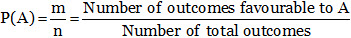
It is obvious that 0 ≤ m ≤ n. If an event A is certain to happen, then m = n, thus P(A) = 1.
If A is impossible to happen, then m = 0 and so P(A) = 0. Hence we conclude that 0 ≤ P(A) ≤ 1. Further, if  denotes negative of A i.e. event that A doesn’t happen, then for above cases m, n; we shall have
.jpg)
.jpg)
Notations: For two events A and B,
A′ or or AC stands for the non-occurrence or negation of A.
A ∪ B stands for the occurrence of at least one of A and B.
A ∩ B stands for the simultaneous occurrence of A and B.
A′ ∩ B′ stands for the non-occurrence of both A and B.
A ⊆ B stands for “the occurrence of A implies occurrence of B”.
Problems based on Combination and Permutation
(1) Problems based on combination or selection:
To solve such kind of problems, we use nCr = n!/(r!(n –r)!)
(2) Problems based on permutation or arrangement:
To solve such kind of problems, we use nPr = n!/(r!(n – r)!)
Odds in favour and odds Against an Event
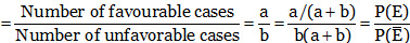
Odds in favour of an event E
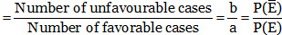
Odds against an event E
Addition Theorems on Probability:
Notations:
P(AB) or P(A ∪ B) = Probability of happening of A or B
= Probability of happening of the events A or B or both
= Probability of occurrence of at least one event A or B
P(AB) or P(A ∩ B) = Probability of happening of events A and B together.
When events are not mutually exclusive:
If A and B are two events which are not mutually exclusive, then
P(A ∪ B) = P(A) + P(B) – P(A ∩ B)
or P(A + B) = P(A) + P(B) – P(AB)
For any three events A, B, C
P(A ∪ B ∪C) = P(A) + P(B) + P(C) – P(A ∩ B) – P(B ∩ C) – P(C ∩ A) + P(A ∩ B ∩ C)
or P(A + B + C) = P(A) + P(B) + P(C) – P(AB) – P(BC) – P(CA) + P(ABC)
(1) When events are mutually exclusive:
If A and B are mutually exclusive events, then
n(A ∩ B) = 0 ⇒ P(A ∩ B) = 0
∴ P(A ∪ B) = P(A) + P(B)
For any three events A, B, C which are mutually exclusive,
P(A ∩ B) = P(B ∩ C) = P(C ∩ A) = P(A ∩ B ∩ C) = 0
∴ P(A ∪C) = P(A) + P(B) + P(C)
The probability of happening of any one of several mutually exclusive events is equal to the sum of their probabilities, i.e. if A1, A2, ... An are mutually exclusive events, then
P(A1 + A2 + ... + An) = P(A1) + P(A2) + ... + P(An)
i.e. P(Σ Ai) = ΣP(A)
(2) When events are independent:
If A and B are independent events, then
P(A ∩ B) = P(A).P(B)
∴ P(A∪B) = P(A) + P(B) – P(A).P(B)
(3) Some other theorems:
(i) Let A and B be two events associated with a random experiment, then
(a) 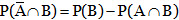
(b) .jpg)
If B ⊂A, then
(a) .jpg)
(b) P(B) ≤ P(A)
Similarly if A ⊂ B, then
(a) .jpg)
(b) P(A) ≤ P(B)
Probability of occurrence of neither A nor B is

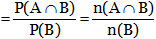
Conditional Probability
► Let A and B be two events associated with a random experiment. Then, the probability of occurrence of A under the condition that B has already occurred and P(B) ≠ 0, is called the conditional probability and it is denoted by P(A/B).
► Thus, P(A/B) = Probability of occurrence of A, given that B has already happened.
► Sometimes, P(A/B) is also used to denote the probability of occurrence of A when B occurs. Similarly, P(B/A) is used to denote the probability of occurrence of B when A occurs.
(1) Multiplication Theorems on Probability
(i) If A and B are two events associated with a random experiment, then
P(A ∩ B) = P(A).P(B/A), If P(A) ≠ 0 or P(A ∩ B) = P(B).P(A/B), if P(B) ≠ 0.
(ii) Multiplication theorems for independent events: If A and B are independent events associated with a random experiment, then P(A ∩ B) = P(A).P(B) i.e., the probability of simultaneous occurrence of two independent events is equal to the product of their probabilities. By multiplication theorem, we have P(A ∩ B) = P(A).P(B/A). Since A and B are independent events, therefore P(B/A) = P(B). Hence, P(A ∩ B) = P(A).P(B)
(2) Probability of at least one of the n independent events:
If p1, p2¸ p3, ... pn e the probabilities of happening of n independent events A1, A2, A3, ... An respectively, then
Probability of happening none of them
.jpg)
.jpg)
= (1 – p1) (1 – p2) (1 – p3) … (1 – pn)
Probability of happening at least one of them
= P(A1 ∪ A2 ∪ A3 … ∪ An)
.jpg)
= 1 – (1 – p1) (1 – p2) (1 – p3) … (1 – pn)
Probability of happening of first event and not happening of the remaining
.jpg)
= p1 (1 – p2) (1 – p3) … (1 – pn)
Total Probability and Baye’s Rule
The Law of Total Probability:
► Let S be the sample space and let E1, E2, ... En be n mutually exclusive and exhaustive events associated with a random experiment. If A is any event which occurs with E1 or E3 or … or En, then
P(A) = P(E1)P(A/E1) + P(E2)P(A/E2) + ... + P(En)P(A/En)
Baye’s rule:
► Let S be a sample space and E1, E2, ... En be n mutually exclusive events such that  and P(Ei) > 0 for i = 1, 2, ……, n. We can think of (Ei’s as the causes that lead to the outcome of an experiment. The probabilities P(Ei), i = 1, 2, ….., n are called prior probabilities. Suppose the experiment results in an outcome of event A, where P(A) > 0. We have to find the probability that the observed event A was due to cause Ei, that is, we seek the conditional probability P(Ei/A). These probabilities are called posterior probabilities, given by Baye’s rule as
.jpg)
Binomial Distribution
(1) Geometrical method for probability:
When the number of points in the sample space is infinite, it becomes difficult to apply classical definition of probability.
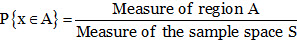
where measure stands for length, area or volume depending upon whether S is a one-dimensional, two-dimensional or three-dimensional region.
(2) Probability distribution:
Let S be a sample space. A random variable X is a function from the set S to R, the set of real numbers.
For example, the sample space for a throw of a pair of dice is
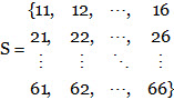
Let X be the sum of numbers on the dice. Then X(12) = 3, X(43) = 7, etc. Also, {X = 7} is the event {61, 52, 43, 34, 25, 16}. In general, if X is a random variable defined on the sample space S and r is a real number, then {X = r} is an event.
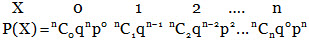
If the random variable X takes n distinct values x1, x2, ..., xn then {X = x1}, {X = x2}, ..., {X = xn} are mutually exclusive and exhaustive events.
.jpg)
Now, since (X = xi) is an event, we can talk of P(X = xi). If P(X = xi) = P(1 ≤ i ≤ n), then the system of numbers. .jpg) is said to be the probability distribution of the random variable X.
is said to be the probability distribution of the random variable X.
The expectation (mean) of the random variable X is defined as .jpg) and the variance of X is defined as
and the variance of X is defined as
.jpg)
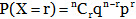
(3) Binomial probability distribution:
A random variable X which takes values 0, 1, 2, …, n is said to follow binomial distribution if its probability distribution function is given by P(X = r) = nCrprqn–r, r = 0,1,2,…,n
where p, q > 0 such that p + q = 1.
The notation X ~ B(n, p) is generally used to denote that the random variable X follows binomial distribution with parameters n and p.
We have P(X = 0) + P(X = 1)+ ... +P(X = n) .
= nC0p0qn–0 + nC1p1qn–1 + ... + nCnpnqn–n = (p + q)n = 1n = 1
Now probability of
(a) Occurrence of the event exactly r times
(b) Occurrence of the event at least r times
.jpg)
(c) Occurrence of the event at the most r times
.jpg)
If the probability of happening of an event in one trial be p, then the probability of successive happening of that event in r trials is pr.
If n trials constitute an experiment and the experiment is repeated N times, then the frequencies of 0, 1, 2, …, n successes are given by N.P(X = 0), N.P(X = 1), N.P(X = 2), ..., N.P(X = n).
(i) Mean and variance of the binomial distribution:
The binomial probability distribution is
The mean of this distribution is
.jpg)
The variance of the Binomial distribution is σ2 = npq and the standard deviation is σ = √(npq).
(ii) Use of multinomial expansion:
If a die has m faces marked with the numbers 1, 2, 3, …. m and if such n dice are thrown, then the probability that the sum of the numbers exhibited on the upper faces equal to p is given by the coefficient of xp in the expansion of 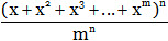 .
.
(4) The poisson distribution:
Let X be a discrete random variable which can take on the values 0, 1, 2,... such that the probability function of X is given by
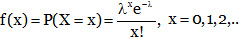
where λ is a given positive constant. This distribution is called the Poisson distribution and a random variable having this distribution is said to be Poisson distributed.
Points at the Glance
► Independent events are always taken from different experiments, while mutually exclusive events are taken from a single experiment.
► Independent events can happen together while mutually exclusive events cannot happen together.
► Independent events are connected by the word “and” but mutually exclusive events are connected by the word “or”.
► Number of exhaustive cases of tossing n coins simultaneously (or of tossing a coin n times) = 2n.
► Number of exhaustive cases of throwing n dice simultaneously (or throwing one dice n times) = 6n.
Probability Regarding n Letters and Their Envelopes
If n letters corresponding to n envelopes are placed in the envelopes at random, then
Probability that all letters are in right envelopes = 1/n!.
Probability that all letters are not in right envelopes = 1 – (1/n!)
Probability that no letter is in right envelopes 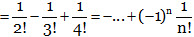
Probability that exactly r letters are in right envelopes .jpg)
If odds in favour of an event are a : b, then the probability of the occurrence of that event is a/(a + b) and the probability of non-occurrence of that event is b/(a + b).
If odds against an event are a : b, then the probability of the occurrence of that event is b/(a + b) and the probability of non-occurrence of that event is a/(a + b).
Let A, B, and C are three arbitrary events. Then
Verbal description of event Equivalent set theoretic notation
Only A occurs – 
Both A and B, but not C occur – .jpg)
All the three events occur – A ∩ B ∩ C
At least one occurs – A ∪ B ∪ C
At least two occur – (A ∩ B) ∪ (B ∩ C) ∪ (A ∩ C)
One and no more occurs – 
Exactly two of A, B and C occur – .jpg)
None occurs – .jpg)
Not more than two occur – (A ∩ B) ∪ (B ∩ C) ∪ (A ∩ C) ∪ (A ∩ B ∩ C)
Exactly one of A and B occurs – .jpg)